MinDE System with Mesoscopic Simulator¶

Fange D, Elf J (2006) Noise-Induced Min Phenotypes in E. coli. PLoS Comput Biol 2(6): e80. doi:10.1371/journal.pcbi.0020080

[1]:

%matplotlib inline
from ecell4 import *
from ecell4_base.core import *
from ecell4_base import meso

Declaring Species and ReactionRules:

[2]:

with species_attributes():
    D | DE | {"D": 0.01, "location": "M"}
    D_ADP | D_ATP | E | {"D": 2.5, "location": "C"}

with reaction_rules():
    D_ATP + M > D | 0.0125
    D_ATP + D > D + D | 9e+6 * (1e+15 / N_A)
    D + E > DE | 5.58e+7 * (1e+15 / N_A)
    DE > D_ADP + E | 0.7
    D_ADP > D_ATP | 0.5

m = get_model()

Make a World. The second argument, 0.05, means its subvolume length:

[3]:

w = meso.World(Real3(4.6, 1.1, 1.1), 0.05)
w.bind_to(m)

Make a structures. Species C is for cytoplasm, and M is for membrane:

[4]:

rod = Rod(3.5, 0.55, w.edge_lengths() * 0.5)
w.add_structure(Species("C"), rod)
w.add_structure(Species("M"), rod.surface())

Throw-in molecules:

[5]:

w.add_molecules(Species("D_ATP"), 2001)
w.add_molecules(Species("D_ADP"), 2001)
w.add_molecules(Species("E"), 1040)

Run a simulation for 120 seconds. Two Observers below are for logging. obs1 logs only the number of molecules, and obs2 does a whole state of the World.

[6]:

sim = meso.Simulator(w)
obs1 = FixedIntervalNumberObserver(0.1, [sp.serial() for sp in m.list_species()])
obs2 = FixedIntervalHDF5Observer(1.0, 'minde%03d.h5')

[7]:

duration = 120
sim.run(duration, (obs1, obs2))

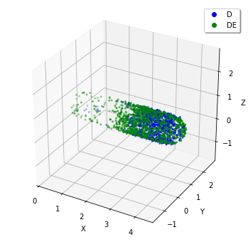
Visualize the final state of the World:

[8]:

plotting.plot_world(w, species_list=('D', 'DE'))

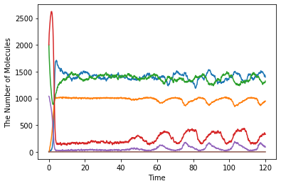
Plot a time course of the number of molecules:

[9]:

show(obs1)

[10]:

plotting.plot_movie(obs2, species_list=('D', 'DE'))

[ ]:

← Lotka-Volterra 2D MinDE System with... →