See also
This page was generated from tutorials/tutorial08.ipynb.
Download the Jupyter Notebook for this section: tutorial08.ipynb. View in nbviewer.
8. More about 1. Brief Tour of E-Cell4 Simulations
Once you read through 1. Brief Tour of E-Cell4 Simulations, it is NOT difficult to use World and Simulator. volume and {'C': 60} is equivalent of the World and solver is the Simulator below.
[1]:
%matplotlib inline
from ecell4.prelude import *

with reaction_rules():
    A + B == C | (0.01, 0.3)

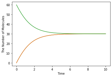
run_simulation(10.0, {'C': 60}, volume=1.0)

Here we give you a breakdown for run_simulation. run_simulation use ODE simulator by default, so we create ode.World step by step.
8.1. Creating ODEWorld
You can create World like this.
[2]:
from ecell4_base.core import *
from ecell4_base import *
[3]:
w = ode.World(Real3(1, 1, 1))
Real3 is a coordinate vector. In this example, the first argument for ode.World constructor is a cube. Note that you can NOT use volume for ode.World argument, like run_simulation argument.
Now you created a cube box for simulation, next let’s throw molecules into the cube.
[4]:
w = ode.World(Real3(1, 1, 1))
w.add_molecules(Species('C'), 60)
print(w.t(), w.num_molecules(Species('C')))  # must return (0.0, 60)
0.0 60
Use add_molecules to add molecules, remove_molecules to remove molecules, num_molecules to know the number of molecules. First argument for each method is the Species you want to know. You can get current time by t method. However the number of molecules in ODE solver is real number, in these _molecules functions work only for integer number. When you handle real numbers in ODE, use set_value and get_value.
8.2. How to Use Real3
Before the detail of Simulator, we explaing more about Real3.
[5]:
pos = Real3(1, 2, 3)
print(pos)  # must print like <ecell4.core.Real3 object at 0x7f44e118b9c0>
print(tuple(pos))  # must print (1.0, 2.0, 3.0)
<ecell4_base.core.Real3 object at 0x151df81bf260>
(1.0, 2.0, 3.0)
You can not print the contents in Real3 object directly. You need to convert Real3 to Python tuple or list once.
[6]:
pos1 = Real3(1, 1, 1)
x, y, z = pos[0], pos[1], pos[2]
pos2 = pos1 + pos1
pos3 = pos1 * 3
pos4 = pos1 / 5
print(length(pos1))  # must print 1.73205080757
print(dot_product(pos1, pos3))  # must print 9.0
1.7320508075688772
9.0
You can use basic function like dot_product. Of course, you can convert Real3 to numpy array too.
[7]:
import numpy
a = numpy.asarray(tuple(Real3(1, 2, 3)))
print(a)  # must print [ 1.  2.  3.]
[1. 2. 3.]
Integer3 represents a triplet of integers.
[8]:
g = Integer3(1, 2, 3)
print(tuple(g))
(1, 2, 3)
Of course, you can also apply simple arithmetics to Integer3.
[9]:
print(tuple(Integer3(1, 2, 3) + Integer3(4, 5, 6)))  # => (5, 7, 9)
print(tuple(Integer3(4, 5, 6) - Integer3(1, 2, 3)))  # => (3, 3, 3)
print(tuple(Integer3(1, 2, 3) * 2))  # => (2, 4, 6)
print(dot_product(Integer3(1, 2, 3), Integer3(4, 5, 6)))  # => 32
print(length(Integer3(1, 2, 3)))  # => 3.74165738677
(5, 7, 9)
(3, 3, 3)
(2, 4, 6)
32
3.7416573867739413
8.3. Creating and Running ODE Simulator
You can create a Simulator with Model and World like
[10]:
with reaction_rules():
    A + B > C | 0.01  # equivalent to create_binding_reaction_rule
    C > A + B | 0.3   # equivalent to create_unbinding_reaction_rule

m = get_model()

sim = ode.Simulator(w, m)
sim.run(10.0)
then call run method, the simulation will run. In this example the simulation runs for 10 seconds.
You can check the state of the World like this.
[11]:
print(w.t(), w.num_molecules(Species('C'))) # must return (10.0, 30)
10.0 30
You can see that the number of the Species C decreases from 60 to 30.
World describes the state at a timepoint, so you can NOT tack the transition during the simulation with the World. To obtain the time-series result, use Observer.
[12]:
w = ode.World(Real3(1, 1, 1))
w.add_molecules(Species('C'), 60)
sim = ode.Simulator(w, m)

obs = FixedIntervalNumberObserver(0.1, ('A', 'C'))
sim.run(10.0, obs)
print(obs.data())  # must return [[0.0, 0.0, 60.0], ..., [10.0, 29.994446899691276, 30.005553100308752]]
[[0.0, 0.0, 60.0], [0.1, 1.7722206143224584, 58.22777938567754], [0.2, 3.4860124975248006, 56.51398750247521], [0.30000000000000004, 5.137633294323578, 54.862366705676436], [0.4, 6.7240908315276045, 53.27590916847241], [0.5, 8.2431297778128, 51.75687022218721], [0.6000000000000001, 9.693203786964157, 50.30679621303585], [0.7000000000000001, 11.073435610343822, 48.926564389656185], [0.8, 12.383567710238625, 47.61643228976138], [0.9, 13.623905934263576, 46.37609406573643], [1.0, 14.795258697983998, 45.204741302016004], [1.1, 15.898873915953542, 44.101126084046456], [1.2000000000000002, 16.936375649258018, 43.06362435074198], [1.3, 17.909702127696086, 42.090297872303914], [1.4000000000000001, 18.821046480898254, 41.17895351910174], [1.5, 19.672801194656238, 40.32719880534375], [1.6, 20.467507011344757, 39.532492988655235], [1.7000000000000002, 21.207806726765288, 38.7921932732347], [1.8, 21.896404106006866, 38.10359589399312], [1.9000000000000001, 22.53602795042438, 37.4639720495756], [2.0, 23.129401196247105, 36.87059880375288], [2.1, 23.679214810305954, 36.320785189694035], [2.2, 24.188106166226664, 35.81189383377333], [2.3000000000000003, 24.6586415307847, 35.341358469215294], [2.4000000000000004, 25.093302260285835, 34.906697739714154], [2.5, 25.494474296223075, 34.505525703776904], [2.6, 25.864440553798364, 34.13555944620162], [2.7, 26.205375812342282, 33.7946241876577], [2.8000000000000003, 26.519343739941075, 33.480656260058915], [2.9000000000000004, 26.808295712922448, 33.19170428707754], [3.0, 27.074071122047478, 32.925928877952515], [3.1, 27.318398889554317, 32.68160111044567], [3.2, 27.54289995329749, 32.45710004670249], [3.3000000000000003, 27.749090505157007, 32.250909494842965], [3.4000000000000004, 27.93838580001201, 32.06161419998797], [3.5, 28.11210437846467, 31.887895621535307], [3.6, 28.27147257094361, 31.728527429056367], [3.7, 28.41762917272733, 31.582370827272648], [3.8000000000000003, 28.551630198838193, 31.448369801161785], [3.9000000000000004, 28.674453644762753, 31.325546355237226], [4.0, 28.78700419370472, 31.212995806295257], [4.1000000000000005, 28.890117823751574, 31.109882176248405], [4.2, 28.98456627912797, 31.015433720872007], [4.3, 29.071061378816175, 30.928938621183804], [4.4, 29.150259143439115, 30.849740856560864], [4.5, 29.222763727609138, 30.77723627239084], [4.6000000000000005, 29.289131150117587, 30.71086884988239], [4.7, 29.349872818534465, 30.650127181465514], [4.800000000000001, 29.40545884814348, 30.5945411518565], [4.9, 29.456321177785775, 30.543678822214204], [5.0, 29.502856487234418, 30.49714351276556], [5.1000000000000005, 29.545428922270702, 30.454571077729277], [5.2, 29.584372634768023, 30.415627365231956], [5.300000000000001, 29.619994145881115, 30.380005854118863], [5.4, 29.652574540951854, 30.347425459048125], [5.5, 29.68237150503112, 30.317628494968858], [5.6000000000000005, 29.709621208023663, 30.290378791976316], [5.7, 29.73454004842796, 30.26545995157202], [5.800000000000001, 29.757326264497603, 30.24267373550238], [5.9, 29.77816142142091, 30.22183857857907], [6.0, 29.797211782822988, 30.202788217176995], [6.1000000000000005, 29.814629574557085, 30.185370425442898], [6.2, 29.830554148384813, 30.16944585161517], [6.300000000000001, 29.84511305275851, 30.154886947241472], [6.4, 29.858423017523837, 30.141576982476145], [6.5, 29.870590858963563, 30.12940914103642], [6.6000000000000005, 29.88171431121031, 30.118285688789673], [6.7, 29.891882789671147, 30.108117210328835], [6.800000000000001, 29.901178091733776, 30.098821908266206], [6.9, 29.909675039664805, 30.090324960335177], [7.0, 29.917442070267278, 30.082557929732705], [7.1000000000000005, 29.92454177553783, 30.075458224462153], [7.2, 29.931031398254603, 30.06896860174538], [7.300000000000001, 29.9369632861354, 30.063036713864584], [7.4, 29.942385307931307, 30.057614692068675], [7.5, 29.94734123456418, 30.0526587654358], [7.6000000000000005, 29.951871088176286, 30.048128911823696], [7.7, 29.95601146173637, 30.043988538263612], [7.800000000000001, 29.9597958116382, 30.04020418836178], [7.9, 29.963254725533886, 30.036745274466096], [8.0, 29.966416167464857, 30.033583832535125], [8.1, 29.969305702187025, 30.030694297812957], [8.200000000000001, 29.971946700432824, 30.02805329956716], [8.3, 29.974360526710818, 30.025639473289164], [8.4, 29.976566711112177, 30.023433288887805], [8.5, 29.978583106472595, 30.021416893527388], [8.6, 29.9804260321266, 30.01957396787338], [8.700000000000001, 29.98211040538864, 30.017889594611344], [8.8, 29.98364986180096, 30.016350138199023], [8.9, 29.985056865101367, 30.014943134898616], [9.0, 29.98634280778428, 30.013657192215703], [9.1, 29.987518103055105, 30.012481896944877], [9.200000000000001, 29.988592268910782, 30.0114077310892], [9.3, 29.98957400501743, 30.01042599498255], [9.4, 29.990471262999563, 30.00952873700042], [9.5, 29.9912913107032, 30.008708689296782], [9.600000000000001, 29.9920407909477, 30.00795920905228], [9.700000000000001, 29.992725775237364, 30.007274224762618], [9.8, 29.993351812863917, 30.006648187136065], [9.9, 29.993923975794377, 30.006076024205605], [10.0, 29.994446899704982, 30.005553100295]]
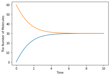
There are several types of Observers for E-Cell4. FixedIntervalNumberObserver is the simplest Observer to obtain the time-series result. As its name suggests, this Observer records the number of molecules for each time-step. The 1st argument is the time-step, the 2nd argument is the molecule types. You can check the result with data method, but there is a shortcut for this.
[13]:
show(obs)

This plots the time-series result easily.
We explained the internal of run_simulation function. When you change the World after creating the Simulator, you need to indicate it to Simulator. So do NOT forget to call sim.initialize() after that.
8.4. Switching the Solver
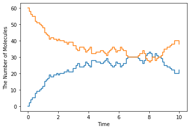
It is NOT difficult to switch the solver to stochastic method, as we showed run_simulation.
[14]:
from ecell4 import *

with reaction_rules():
    A + B == C | (0.01, 0.3)

m = get_model()

# ode.World -> gillespie.World
w = gillespie.World(Real3(1, 1, 1))
w.add_molecules(Species('C'), 60)

# ode.Simulator -> gillespie.Simulator
sim = gillespie.Simulator(w, m)
obs = FixedIntervalNumberObserver(0.1, ('A', 'C'))
sim.run(10.0, obs)

show(obs, step=True)

World and Simulator never change the Model itself, so you can switch several Simulators for one Model.