5. How to Log and Visualize Simulations¶

5.1. Logging Simulations with Observers¶

E-Cell4 provides special classes for logging, named Observer. Observer class is given when you call the run function of Simulator.

[2]:

def create_simulator(f=gillespie.Factory()):
    m = NetworkModel()
    A, B, C = Species('A', 0.005, 1), Species('B', 0.005, 1), Species('C', 0.005, 1)
    m.add_species_attribute(A)
    m.add_species_attribute(B)
    m.add_species_attribute(C)
    m.add_reaction_rule(create_binding_reaction_rule(A, B, C, 0.01))
    m.add_reaction_rule(create_unbinding_reaction_rule(C, A, B, 0.3))

    w = f.world()
    w.bind_to(m)
    w.add_molecules(C, 60)

    sim = f.simulator(w)
    sim.initialize()
    return sim

One of most popular Observer is FixedIntervalNumberObserver, which logs the number of molecules with the given time interval. FixedIntervalNumberObserver requires an interval and a list of serials of Species for logging.

[3]:

obs1 = FixedIntervalNumberObserver(0.1, ['A', 'B', 'C'])
sim = create_simulator()
sim.run(1.0, obs1)

data function of FixedIntervalNumberObserver returns the data logged.

[4]:

print(obs1.data())

[[0.0, 0.0, 0.0, 60.0], [0.1, 6.0, 6.0, 54.0], [0.2, 7.0, 7.0, 53.0], [0.30000000000000004, 10.0, 10.0, 50.0], [0.4, 13.0, 13.0, 47.0], [0.5, 13.0, 13.0, 47.0], [0.6000000000000001, 13.0, 13.0, 47.0], [0.7000000000000001, 14.0, 14.0, 46.0], [0.8, 14.0, 14.0, 46.0], [0.9, 15.0, 15.0, 45.0], [1.0, 16.0, 16.0, 44.0]]

targets() returns a list of Species, which you specified as an argument of the constructor.

[5]:

print([sp.serial() for sp in obs1.targets()])

['A', 'B', 'C']

NumberObserver logs the number of molecules after every steps when a reaction occurs. This observer is useful to log all reactions, but not available for ode.

[6]:

obs1 = NumberObserver(['A', 'B', 'C'])
sim = create_simulator()
sim.run(1.0, obs1)
print(obs1.data())

[[0.0, 0.0, 0.0, 60.0], [0.0046880772084985575, 1.0, 1.0, 59.0], [0.02940433389289125, 2.0, 2.0, 58.0], [0.0424566850969309, 3.0, 3.0, 57.0], [0.056679020913974754, 4.0, 4.0, 56.0], [0.06363561718447702, 5.0, 5.0, 55.0], [0.06628282436583607, 6.0, 6.0, 54.0], [0.14965843277576601, 7.0, 7.0, 53.0], [0.17585986686274913, 8.0, 8.0, 52.0], [0.34117216604734923, 9.0, 9.0, 51.0], [0.3434039354567801, 10.0, 10.0, 50.0], [0.3964706785644159, 11.0, 11.0, 49.0], [0.4299973974400797, 10.0, 10.0, 50.0], [0.4754407324998785, 11.0, 11.0, 49.0], [0.4924264239728917, 12.0, 12.0, 48.0], [0.5615452208142621, 13.0, 13.0, 47.0], [0.5799521557799048, 14.0, 14.0, 46.0], [0.5999770573122667, 13.0, 13.0, 47.0], [0.617181962644011, 14.0, 14.0, 46.0], [0.771123487556924, 15.0, 15.0, 45.0], [0.8527649352650291, 14.0, 14.0, 46.0], [1.0, 14.0, 14.0, 46.0]]

TimingNumberObserver allows you to give the times for logging as an argument of its constructor.

[7]:

obs1 = TimingNumberObserver([0.0, 0.1, 0.2, 0.5, 1.0], ['A', 'B', 'C'])
sim = create_simulator()
sim.run(1.0, obs1)
print(obs1.data())

[[0.0, 0.0, 0.0, 60.0], [0.1, 6.0, 6.0, 54.0], [0.2, 7.0, 7.0, 53.0], [0.5, 12.0, 12.0, 48.0], [1.0, 17.0, 17.0, 43.0]]

run function accepts multile Observers at once.

[8]:

obs1 = NumberObserver(['C'])
obs2 = FixedIntervalNumberObserver(0.1, ['A', 'B'])
sim = create_simulator()
sim.run(1.0, [obs1, obs2])
print(obs1.data())
print(obs2.data())

[[0.0, 60.0], [0.0046880772084985575, 59.0], [0.02940433389289125, 58.0], [0.0424566850969309, 57.0], [0.056679020913974754, 56.0], [0.06363561718447702, 55.0], [0.06628282436583607, 54.0], [0.12593245801241867, 53.0], [0.2021936427813259, 52.0], [0.2544761483060903, 51.0], [0.28758664472519707, 50.0], [0.3350787275656141, 49.0], [0.36976606582502675, 48.0], [0.3732460193898695, 47.0], [0.5040022833539709, 46.0], [0.5763738195435169, 47.0], [0.6425014653528736, 46.0], [0.809322179639534, 45.0], [0.8095585219320289, 44.0], [0.8536384048043809, 45.0], [0.997992921530679, 44.0], [1.0, 44.0]]
[[0.0, 0.0, 0.0], [0.1, 6.0, 6.0], [0.2, 7.0, 7.0], [0.30000000000000004, 10.0, 10.0], [0.4, 13.0, 13.0], [0.5, 13.0, 13.0], [0.6000000000000001, 13.0, 13.0], [0.7000000000000001, 14.0, 14.0], [0.8, 14.0, 14.0], [0.9, 15.0, 15.0], [1.0, 16.0, 16.0]]

FixedIntervalHDF5Observedr logs the whole data in a World to an output file with the fixed interval. Its second argument is a prefix for output filenames. filename() returns the name of a file scheduled to be saved next. At most one format string like %02d is allowed to use a step count in the file name. When you do not use the format string, it overwrites the latest data to the file.

[9]:

obs1 = FixedIntervalHDF5Observer(0.2, 'test%02d.h5')
print(obs1.filename())
sim = create_simulator()
sim.run(1.0, obs1) # Now you have steped 5 (1.0/0.2) times
print(obs1.filename())

test00.h5
test06.h5

[10]:

w = load_world('test05.h5')
print(w.t(), w.num_molecules(Species('C')))

1.0 46

The usage of FixedIntervalCSVObserver is almost same with that of FixedIntervalHDF5Observer. It saves positions (x, y, z) of particles with the radius (r) and serial number of Species (sid) to a CSV file.

[11]:

obs1 = FixedIntervalCSVObserver(0.2, "test%02d.csv")
print(obs1.filename())
sim = create_simulator()
sim.run(1.0, obs1)
print(obs1.filename())

test00.csv
test06.csv

Here is the first 10 lines in the output CSV file.

[12]:

print(''.join(open("test05.csv").readlines()[: 10]))

x,y,z,r,sid
0.698028,0.576404,0.909806,0,0
0.718767,0.595254,0.776376,0,0
0.0871218,0.403749,0.889247,0,0
0.620976,0.317304,0.73291,0,0
0.422875,0.756634,0.486491,0,0
0.489729,0.869672,0.604034,0,0
0.27081,0.184816,0.475873,0,0
0.155155,0.842252,0.444279,0,0
0.270323,0.236893,0.544951,0,0

For particle simulations, E-Cell4 also provides Observer to trace a trajectory of a molecule, named FixedIntervalTrajectoryObserver. When no ParticleID is specified, it logs all the trajectories. Once some ParticleID is lost for the reaction during a simulation, it just stop to trace the particle any more.

[13]:

sim = create_simulator(spatiocyte.Factory(0.005))
obs1 = FixedIntervalTrajectoryObserver(0.01)
sim.run(0.1, obs1)

[14]:

print([tuple(pos) for pos in obs1.data()[0]])

[(0.563382640840131, 0.9901557116602082, 0.965), (0.6205374015050719, 1.0478907385791707, 0.935), (0.59604250407724, 1.0074762197358968, 0.915), (0.6776921621700127, 1.0594377439629632, 1.185), (0.751176854453508, 1.0392304845413263, 1.18), (0.8328265125462806, 0.9612881982007269, 1.225), (0.8899812732112214, 1.0421172358872746, 1.375), (0.751176854453508, 1.1344932789576145, 1.305), (0.9226411364483306, 1.0334569818494301, 1.2), (0.7348469228349536, 1.0738715006927038, 1.51), (0.8164965809277261, 1.0132497224277932, 1.605)]

Generally, World assumes a periodic boundary for each plane. To avoid the big jump of a particle at the edge due to the boundary condition, FixedIntervalTrajectoryObserver tries to keep the shift of positions. Thus, the positions stored in the Observer are not necessarily limited in the cuboid given for the World. To track the diffusion over the boundary condition accurately, the step interval for logging must be small enough. Of course, you can disable this option. See help(FixedIntervalTrajectoryObserver).

5.2. Visualization of Data Logged¶

In this section, we explain the visualization tools for data logged by Observer.

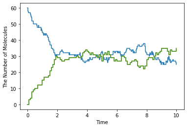
Firstly, for time course data, plotting.plot_number_observer plots the data provided by NumberObserver, FixedIntervalNumberObserver and TimingNumberObserver. For the detailed usage of plotting.plot_number_observer, see help(plotting.plot_number_observer).

[15]:

obs1 = NumberObserver(['C'])
obs2 = FixedIntervalNumberObserver(0.1, ['A', 'B'])
sim = create_simulator()
sim.run(10.0, [obs1, obs2])

[16]:

plotting.plot_number_observer(obs1, obs2, step=True)

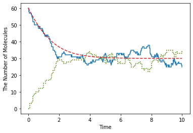
You can set the style for plotting, and even add an arbitrary function to plot.

[17]:

plotting.plot_number_observer(obs1, '-', obs2, ':', lambda t: 60 * (1 + 2 * math.exp(-0.9 * t)) / (2 + math.exp(-0.9 * t)), '--', step=True)

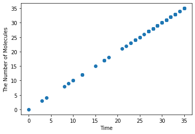
Plotting in the phase plane is also available by specifing the x-axis and y-axis.

[18]:

plotting.plot_number_observer(obs2, 'o', x='A', y='B')

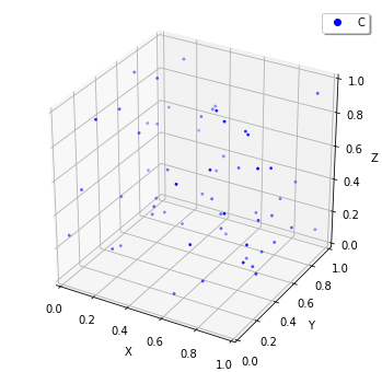
For spatial simulations, to visualize the state of World, plotting.plot_world is available. This function plots the points of particles in three-dimensional volume in the interactive way. You can save the image by clicking a right button on the drawing region.

[19]:

sim = create_simulator(spatiocyte.Factory(0.005))
plotting.plot_world(sim.world())

You can also make a movie from a series of HDF5 files, given as a FixedIntervalHDF5Observer. plotting.plot_movie requires an extra library, ffmpeg.

[20]:

sim = create_simulator(spatiocyte.Factory(0.005))
obs1 = FixedIntervalHDF5Observer(0.02, 'test%02d.h5')
sim.run(1.0, obs1)
plotting.plot_movie(obs1)

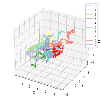
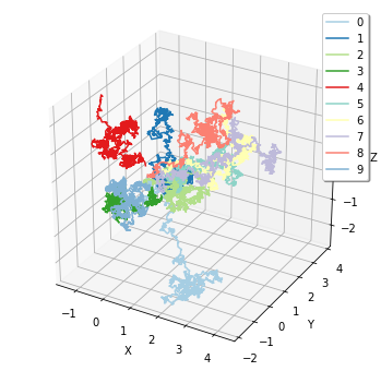
Finally, corresponding to FixedIntervalTrajectoryObserver, plotting.plot_trajectory provides a visualization of particle trajectories.

[21]:

sim = create_simulator(spatiocyte.Factory(0.005))
obs1 = FixedIntervalTrajectoryObserver(1e-3)
sim.run(1, obs1)
plotting.plot_trajectory(obs1)

show internally calls these plotting functions corresponding to the given observer. Thus, you can do simply as follows:

[22]:

show(obs1)