2. How to Build a Model¶

2.1. Species¶

Species can be generated by giving its name:

[2]:

sp1 = Species("A")
print(sp1.serial())

A

There are some naming conventions for the name of Species. This naming convention requires careful use of special symbols (e.g. parenthesis (), dot ., underbar _), numbers and blank.

Species has a set of APIs for handling its attributes:

[3]:

sp1.set_attribute("radius", 0.005)
sp1.set_attribute("D", 1)
sp1.set_attribute("location", "cytoplasm")
print(sp1.has_attribute("radius"))
print(sp1.get_attribute("radius"))
print(sp1.get_attribute("radius").magnitude)
print(sp1.get_attribute("radius").units)
print(sp1.has_attribute("location"))
print(sp1.get_attribute("location"))
sp1.remove_attribute("radius")
print(sp1.has_attribute("radius"))

True
<ecell4_base.core.Quantity_Real object at 0x149ce5fde618>
0.005

True
cytoplasm
False

The arguments in set_attribute is the name of attribute and its value. The name of an attribute is given as a string, and its value is a string, integer, float, or boolean. get_attribute returns the value set. For an integer or float attribute, get_attribute returns a quantity object, which is a pair of value (magnitude) and unit (units).

There is a shortcut to set the attributes above at once because radius, D (a diffusion coefficient) and location are frequently used.

[4]:

sp1 = Species("A", 0.005, 1, "cytoplasm")  # serial, radius, D, location

The equality between Species is just evaluated based on their serial:

[5]:

print(Species("A") == Species("B"))
print(Species("A") == Species("A"))

False
True

A Species consists of one or more UnitSpecies:

[6]:

sp1 = Species()
usp1 = UnitSpecies("C")
print(usp1.serial())
sp1.add_unit(usp1)
sp1.add_unit(UnitSpecies("A"))
sp1.add_unit(UnitSpecies("B"))
print(sp1.serial(), len(sp1.units()))

C
C.A.B 3

A Species can be reproduced from its serial. In the serial, all UnitSpecies are joined with the separator, dot .. The order of UnitSpecies affects the Species comparison.

[7]:

sp1 = Species("C.A.B")
print(sp1.serial())
print(Species("A.B.C") == Species("C.A.B"))
print(Species("A.B.C") == Species("A.B.C"))

C.A.B
False
True

UnitSpecies can have sites. Sites consists of a name, state and bond, and are sorted automatically in UnitSpecies. name must be unique in a UnitSpecies. All the value have to be string. Do not include parenthesis, dot and blank, and not start from numbers except for bond.

[8]:

usp1 = UnitSpecies("A")
usp1.add_site("us", "u", "")
usp1.add_site("ps", "p", "_")
usp1.add_site("bs", "", "_")
print(usp1.serial())

A(bs^_,ps=p^_,us=u)

UnitSpecies can be also reproduced from its serial. Please be careful with the order of sites where a site with a state must be placed after sites with no state specification:

[9]:

usp1 = UnitSpecies()
usp1.deserialize("A(bs^_, us=u, ps=p^_)")
print(usp1.serial())

A(bs^_,ps=p^_,us=u)

Of course, a site of UnitSpecies is available even in Species’ serial.

[10]:

sp1 = Species("A(bs^1, ps=u).A(bs, ps=p^1)")
print(sp1.serial())
print(len(sp1.units()))

A(bs^1, ps=u).A(bs, ps=p^1)
2

The information (UnitSpecies and its site) is used for rule-based modeling. The way of rule-based modeling in E-Cell4 is explained in 7. Introduction of Rule-based Modeling.

2.2. ReactionRule¶

ReactionRule consists of reactants, products and k. reactants and products are a list of Species, and k is a kinetic rate given as a floating number.

[11]:

rr1 = ReactionRule()
rr1.add_reactant(Species("A"))
rr1.add_reactant(Species("B"))
rr1.add_product(Species("C"))
rr1.set_k(1.0)

Here is a binding reaction from A and B to C. In this reaction definition, you don’t need to set attributes to Species. The above series of operations can be written in one line using create_binding_reaction_rule(Species("A"), Species("B"), Species("C"), 1.0).

You can use as_string function to check ReactionRule:

[12]:

rr1 = create_binding_reaction_rule(Species("A"), Species("B"), Species("C"), 1.0)
print(rr1.as_string())

A+B>C|1

You can also provide components to the constructor:

[13]:

rr1 = ReactionRule([Species("A"), Species("B")], [Species("C")], 1.0)
print(rr1.as_string())

A+B>C|1

Basically ReactionRule represents a mass action reaction with the rate k. ode solver also supports rate laws thought it’s under development yet. ode.ODERatelaw is explained in 6. How to Solve ODEs with Rate Law Functions local ipynb readthedocs.

2.3. NetworkModel¶

You have learned how to create some Model components. Next let’s put the components in a Model.

[14]:

sp1 = Species("A", 0.005, 1)
sp2 = Species("B", 0.005, 1)
sp3 = Species("C", 0.01, 0.5)

[15]:

rr1 = create_binding_reaction_rule(Species("A"), Species("B"), Species("C"), 0.01)
rr2 = create_unbinding_reaction_rule(Species("C"), Species("A"), Species("B"), 0.3)

You can put the Species and ReactionRule with add_species_attribute and add_reaction_rule.

[16]:

m1 = NetworkModel()
m1.add_species_attribute(sp1)
m1.add_species_attribute(sp2)
m1.add_species_attribute(sp3)
m1.add_reaction_rule(rr1)
m1.add_reaction_rule(rr2)

Now we have a simple model with the binding and unbinding reactions. You can use species_attributes and reaction_rules to check the Model.

[17]:

print([sp.serial() for sp in m1.species_attributes()])
print([rr.as_string() for rr in m1.reaction_rules()])

['A', 'B', 'C']
['A+B>C|0.01', 'C>A+B|0.3']

The Species attributes are required for the spatial Model, but not required for the nonspatial Model (i.e. gillespie or ode). The attribute pushed first has higher priority than one pushed later. You can also attribute a Species based on the attributes in a Model.

[18]:

sp1 = Species("A")
print(sp1.has_attribute("radius"))
sp2 = m1.apply_species_attributes(sp1)
print(sp2.has_attribute("radius"))
print(sp2.get_attribute("radius").magnitude)

False
True
0.005

For your information, all functions related to Species, ReactionRule and NetworkModel above are also available on C++ in the same way.

Finally, you can solve this model with run_simulation as explained in 1. Brief Tour of E-Cell4 Simulations :

[19]:

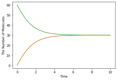
run_simulation(10.0, model=m1, y0={'C': 60})

2.4. Python Utilities to Build a Model¶

As shown in 1. Brief Tour of E-Cell4 Simulations, E-Cell4 also provides the easier way to build a model using with statement:

[20]:

with species_attributes():
    A | B | {'radius': 0.005, 'D': 1}
    C | {'radius': 0.01, 'D': 0.5}

with reaction_rules():
    A + B == C | (0.01, 0.3)

m1 = get_model()

For reversible reactions, == is available. In the with statement, undeclared variables are automaticaly assumed to be a Species. Any Python variables, functions and statement are available even in the with block.

[21]:

from math import log

ka, kd, kf = 0.01, 0.3, 0.1
tau = 10.0

with reaction_rules():
    E0 + S == ES | (ka, kd)

    if tau > 0:
        ES > E1 + P | kf
        E1 > E0 | log(2) / tau
    else:
        ES > E0 + P | kf

m1 = get_model()
del ka, kd, kf, tau

Meanwhile, once some variable is declared even outside the block, you can not use its name as a Species as follows:

[22]:

A = 10

try:
    with reaction_rules():
        A + B == C | (0.01, 0.3)
except Exception as e:
    print(repr(e))

del A

TypeError("Argument 1 must be AnyCallable, ParseObj, InvExp or MulExp. 'int' was given [10].")

This is because A + B == C is evaluated as 10 + B == C due to A = 10.

In the absence of left or right hand side of ReactionRule like synthesis or degradation, you may want to describe like:

with reaction_rules():
    A > | 1.0  # XXX: will raise SyntaxError
    > A | 1.0  # XXX: will raise SyntaxError

However, this is not accepted because of the syntax rule on Python. To describe this case, a special operator, tilde ~, is available. ~ sets a stoichiometric coefficient of the following Species as zero, which means the Species is just ignored in the ReactionRule.

[23]:

with reaction_rules():
    ~A > A | 2.0  # equivalent to `create_synthesis_reaction_rule`
    A > ~A | 1.0  # equivalent to `create_degradation_reaction_rule`

m1 = get_model()
print([rr.as_string() for rr in m1.reaction_rules()])

['>A|2', 'A>|1']

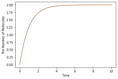
The following Species’ name is not necessarily needed to be the same as others. The model above describes \([A]'=2-1\times[A]\):

[24]:

from math import exp
ret = run_simulation(10.0, model=m1)
ret.plot('-', lambda t: 2.0 * (1 - exp(-t)), '--')

A chain of reactions can be described in one line. To split a line into two or more physical lines, wrap lines in a parenthesis:

[25]:

with reaction_rules():
    (E + S == ES | (0.5, 1.0)
         > E + P | 1.5)

m1 = get_model()
print([rr.as_string() for rr in m1.reaction_rules()])

['E+S>ES|0.5', 'ES>E+S|1', 'ES>E+P|1.5']

The method uses global variables in ecell4.util.decorator (e.g. REACTION_RULES) to cache objects created in the with statement:

[26]:

import ecell4.util.decorator

with reaction_rules():
    A + B == C | (0.01, 0.3)

print(ecell4.util.decorator.REACTION_RULES)  #XXX: Only for debugging
get_model()
print(ecell4.util.decorator.REACTION_RULES)  #XXX: Only for debugging

[<ecell4_base.core.ReactionRule object at 0x149ce5bad378>, <ecell4_base.core.ReactionRule object at 0x149ce5bad1f0>]
[]

Python decorator functions are also available. Decorator functions improve the modularity of the Model.

[27]:

@species_attributes
def attrgen1(radius, D):
    A | B | {'radius': radius, 'D': D}
    C | {'radius': radius * 2, 'D': D * 0.5}

@reaction_rules
def rrgen1(kon, koff):
    A + B == C | (kon, koff)

attrs1 = attrgen1(0.005, 1)
rrs1 = rrgen1(0.01, 0.3)
print(attrs1)
print(rrs1)

[(<ecell4_base.core.Species object at 0x149ce5c1b1b8>, False), (<ecell4_base.core.Species object at 0x149ce5c1b570>, False), (<ecell4_base.core.Species object at 0x149ce5c1b768>, False)]
[<ecell4_base.core.ReactionRule object at 0x149ce5c1bb58>, <ecell4_base.core.ReactionRule object at 0x149ce5c1b260>]

In contrast to the with statement, do not add parentheses after the decorator here. The functions decorated by reaction_rules and species_attributes return a list of ReactionRules and Species respectively. The list can be registered to Model at once by using add_reaction_rules and add_species_attributes.

[28]:

m1 = NetworkModel()
m1.add_species_attributes(attrs1)
m1.add_reaction_rules(rrs1)
print(m1.num_reaction_rules())

2

This method is modular and reusable relative to the way using with statement.

The functions decorated by species_attributes and reaction_rules are also reusable in the with statement.

[29]:

@reaction_rules
def michaelis_menten(S, P, E, ES, kf, kr, kcat):
    S + E == ES | (kf, kr)
    ES > P + E | kcat

with reaction_rules():
    michaelis_menten(K, Kp, KK, KK_K, 0.01, 0.3, 0.15)
    michaelis_menten(Kp, K, PP, PP_Kp, 0.01, 0.3, 0.15)

m1 = get_model()
show(m1)

K + KK > KK_K | 0.01
KK_K > K + KK | 0.3
KK_K > Kp + KK | 0.15
Kp + PP > PP_Kp | 0.01
PP_Kp > Kp + PP | 0.3
PP_Kp > K + PP | 0.15