Mean Square Displacement (MSD)¶

This is a validation for the E-Cell4 library. Here, we test a mean square displacement (MSD) for each simulation algorithms.

[1]:

%matplotlib inline
import matplotlib.pyplot as plt
import numpy
from ecell4.prelude import *

Making a model for all. A single species A is defined. The radius is 5 nm, and the diffusion coefficient is 1um^2/s:

[2]:

radius, D = 0.005, 1
m = NetworkModel()
m.add_species_attribute(Species("A", radius, D))

Create a random number generator, which is used through whole simulations below:

[3]:

rng = GSLRandomNumberGenerator()
rng.seed(0)

Distribution along each axis¶

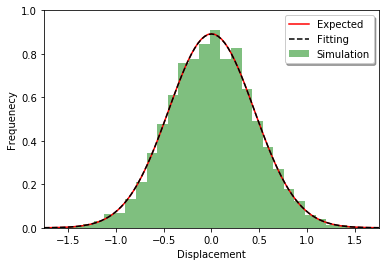
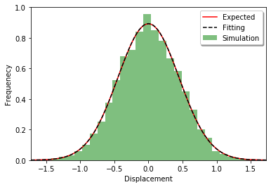
First, a distribution along each axis is tested. The distribution after the time t should follow the normal distribution with mean 0 and variance 2Dt.

[4]:

def plot_displacements(ret):
    distances = []
    for ret_ in ret:
        obs = ret_.observers[1]
        for data in obs.data():
            distances.extend(tuple(data[-1] - data[0]))

    _, bins, _ = plt.hist(distances, bins=30, density=True, facecolor='green', alpha=0.5, label='Simulation')
    xmax = max(abs(bins[0]), abs(bins[-1]))
    x = numpy.linspace(-xmax, +xmax, 101)
    gauss = lambda x, sigmasq: numpy.exp(-0.5 * x * x / sigmasq) / numpy.sqrt(2 * numpy.pi * sigmasq)
    plt.plot(x, gauss(x, 2 * D * duration), 'r-', label='Expected')
    plt.plot(x, gauss(x, sum(numpy.array(distances) ** 2) / len(distances)), 'k--', label='Fitting')
    plt.xlim(x[0], x[-1])
    plt.ylim(0, 1)
    plt.xlabel('Displacement')
    plt.ylabel('Frequenecy')
    plt.legend(loc='best', shadow=True)
    plt.show()

[5]:

duration = 0.1
N = 50
obs = FixedIntervalTrajectoryObserver(0.01)

Simulating with egfrd:

[6]:

ret1 = ensemble_simulations(
    duration, ndiv=1, model=m, y0={'A': N}, observers=obs,
    solver=('egfrd', Integer3(4, 4, 4)), repeat=50)

[7]:

show(ret1[0].observers[1])

[8]:

plot_displacements(ret1)

Simulating with spatiocyte:

[9]:

ret2 = ensemble_simulations(
    duration, ndiv=1, model=m, y0={'A': N}, observers=obs,
    solver=('spatiocyte', radius), repeat=50)

[10]:

plot_displacements(ret2)

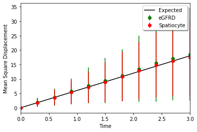
Mean square displacement¶

A mean square displacement after the time t is euqal to the variance above. The one of a diffusion in volume is 6Dt. ecell4.FixedIntervalTrajectoryObserver enables to track a trajectory of a particle over periodic boundaries.

[11]:

def test_mean_square_displacement(ret):
    t = numpy.array(ret[0].observers[1].t())
    sd = []
    for ret_ in ret:
        obs = ret_.observers[1]
        for data in obs.data():
            sd.append(numpy.array([length_sq(pos - data[0]) for pos in data]))
    return (t, numpy.average(sd, axis=0), numpy.std(sd, axis=0))

[12]:

duration = 3.0
N = 50
obs = FixedIntervalTrajectoryObserver(0.01)

Simulating with egfrd:

[13]:

ret1 = ensemble_simulations(
    duration, ndiv=1, model=m, y0={'A': N}, observers=obs,
    solver=('egfrd', Integer3(4, 4, 4)), repeat=10)

[14]:

t, mean1, std1 = test_mean_square_displacement(ret1)

Simulating with spatiocyte:

[15]:

ret2 = ensemble_simulations(
    duration, ndiv=1, model=m, y0={'A': N}, observers=obs,
    solver=('spatiocyte', radius), repeat=10)

[16]:

t, mean2, std2 = test_mean_square_displacement(ret2)

[17]:

plt.plot(t, 6 * D * t, 'k-', label="Expected")
plt.errorbar(t[::30], mean1[::30], yerr=std1[::30], fmt='go', label="eGFRD")
plt.errorbar(t[::30], mean2[::30], yerr=std2[::30], fmt='ro', label="Spatiocyte")
plt.xlim(t[0], t[-1])
plt.legend(loc="best", shadow=True)
plt.xlabel("Time")
plt.ylabel("Mean Square Displacement")
plt.show()

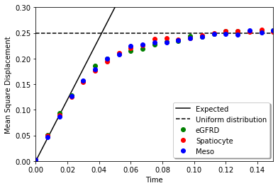
Mean square displacement in a cube¶

Here, we test a mean square diplacement in a cube. For the periodic boundaries, particles cannot escape from World, and thus the displacement for each axis is less than a half of the World size. In meso simulations, unlike egfrd and spatiocyte, each molecule doesn’t have its ParticleID. meso is just validated in this condition because FixedIntervalTrajectoryObserver is only available with ParticleID.

[18]:

def multirun(target, job, repeat, method=None, **kwargs):
    from ecell4.extra.ensemble import run_ensemble, genseeds
    from ecell4.util.session import ResultList

    return run_ensemble(target, [list(job) + [genseeds(repeat)]], repeat=repeat, method=method, **kwargs)[0]

[19]:

def singlerun(job, job_id, task_id):
    from ecell4_base.core import AABB, Real3, GSLRandomNumberGenerator
    from ecell4_base.core import FixedIntervalNumberObserver, FixedIntervalTrajectoryObserver
    from ecell4.util.session import get_factory
    from ecell4.extra.ensemble import getseed

    duration, solver, ndiv, myseeds = job
    rndseed = getseed(myseeds, task_id)

    f = get_factory(*solver)
    f.rng(GSLRandomNumberGenerator(rndseed))
    w = f.world(ones())
    L_11, L_2 = 1.0 / 11, 1.0 / 2
    w.bind_to(m)
    NA = 12
    w.add_molecules(Species("A"), NA, AABB(Real3(5, 5, 5) * L_11, Real3(6, 6, 6) * L_11))

    sim = f.simulator(w)

    retval = [sum(length_sq(p.position() - Real3(L_2, L_2, L_2)) for pid, p in w.list_particles_exact(Species("A"))) / NA]
    for i in range(ndiv):
        sim.run(duration / ndiv)
        mean = sum(length_sq(p.position() - Real3(L_2, L_2, L_2)) for pid, p in w.list_particles_exact(Species("A"))) / NA
        retval.append(mean)
    return numpy.array(retval)

[20]:

duration = 0.15
ndiv = 20
t = numpy.linspace(0, duration, ndiv + 1)

Simulating with egfrd:

[21]:

ret1 = multirun(singlerun, job=(duration, ("egfrd", Integer3(4, 4, 4)), ndiv), repeat=50)

[22]:

mean1 = numpy.average(ret1, axis=0)

Simulating with spatiocyte:

[23]:

ret2 = multirun(singlerun, job=(duration, ("spatiocyte", radius), ndiv), repeat=50)

[24]:

mean2 = numpy.average(ret2, axis=0)

Simulating with meso:

[25]:

ret3 = multirun(singlerun, job=(duration, ("meso", Integer3(11, 11, 11)), ndiv), repeat=50)

[26]:

mean3 = numpy.average(ret3, axis=0)

Mean square displacement at the uniform distribution in a cube is calculated as follows:

\(\int_0^1\int_0^1\int_0^1 dxdydz\ (x-0.5)^2+(y-0.5)^2+(z-0.5)^2=3\left[\frac{(x-0.5)^3}{3}\right]_0^1=0.25\)

[27]:

plt.plot(t, 6 * D * t, 'k-', label="Expected")
plt.plot((t[0], t[-1]), (0.25, 0.25), 'k--', label='Uniform distribution')
plt.plot(t, mean1, 'go', label="eGFRD")
plt.plot(t, mean2, 'ro', label="Spatiocyte")
plt.plot(t, mean3, 'bo', label="Meso")
plt.xlim(t[0], t[-1])
plt.ylim(0, 0.3)
plt.legend(loc="best", shadow=True)
plt.xlabel("Time")
plt.ylabel("Mean Square Displacement")
plt.show()

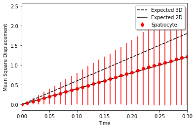
Mean square displacement in 2D¶

Spatial simulation with a structure is only supported by spatiocyte and meso now. Here, mean square displacement on a planar surface is tested for these algorithms.

First, a model is defined with a species A which has the same attributes with above except for the location named M.

[28]:

radius, D = 0.005, 1

m = NetworkModel()
A = Species("A", radius, D, "M")
A.set_attribute("dimension", 2)
m.add_species_attribute(A)
M = Species("M", radius, 0)
M.set_attribute("dimension", 2)
m.add_species_attribute(M)

Mean square displacement of a 2D diffusion must follow 4Dt. The diffusion on a planar surface parallel to yz-plane at the center is tested with spatiocyte.

[29]:

duration = 0.3
N = 50
obs = FixedIntervalTrajectoryObserver(0.01)

Simulating with spatiocyte:

[30]:

ret2 = ensemble_simulations(
    duration, ndiv=1, model=m, y0={'A': N}, observers=obs,
    structures={'M': PlanarSurface(0.5 * ones(), unity(), unitz())},
    solver=('spatiocyte', radius), repeat=50)

[31]:

t, mean2, std2 = test_mean_square_displacement(ret2)

[32]:

plt.plot(t, 6 * D * t, 'k--', label="Expected 3D")
plt.plot(t, 4 * D * t, 'k-', label="Expected 2D")
plt.errorbar(t, mean2, yerr=std2, fmt='ro', label="Spatiocyte")
plt.xlim(t[0], t[-1])
plt.legend(loc="best", shadow=True)
plt.xlabel("Time")
plt.ylabel("Mean Square Displacement")
plt.show()

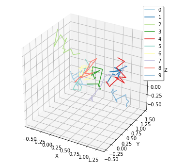
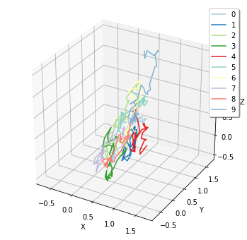
Plottig the trajectory of particles on a surface with spatiocyte:

[33]:

viz.plot_trajectory(ret2[0].observers[1])

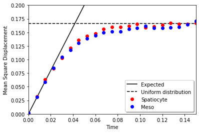
Mean square displacement on a planar surface restricted in a cube by periodic boundaries is compared between meso and spatiocyte.

[34]:

def singlerun(job, job_id, task_id):
    from ecell4_base.core import AABB, Real3, GSLRandomNumberGenerator
    from ecell4_base.core import FixedIntervalNumberObserver, FixedIntervalTrajectoryObserver
    from ecell4.util.session import get_factory
    from ecell4.extra.ensemble import getseed

    duration, solver, ndiv, myseeds = job
    rndseed = getseed(myseeds, task_id)

    f = get_factory(*solver)
    f.rng(GSLRandomNumberGenerator(rndseed))

    w = f.world(ones())
    L_11, L_2 = 1.0 / 11, 1.0 / 2
    w.bind_to(m)
    NA = 12
    w.add_structure(Species("M"), PlanarSurface(0.5 * ones(), unity(), unitz()))
    w.add_molecules(Species("A"), NA, AABB(ones() * 5 * L_11, ones() * 6 * L_11))

    sim = f.simulator(w)

    retval = [sum(length_sq(p.position() - Real3(L_2, L_2, L_2)) for pid, p in w.list_particles_exact(Species("A"))) / NA]
    for i in range(ndiv):
        sim.run(duration / ndiv)
        mean = sum(length_sq(p.position() - Real3(L_2, L_2, L_2)) for pid, p in w.list_particles_exact(Species("A"))) / NA
        retval.append(mean)
    return numpy.array(retval)

[35]:

duration = 0.15
ndiv = 20
t = numpy.linspace(0, duration, ndiv + 1)

Simulating with spatiocyte:

[36]:

ret2 = multirun(singlerun, job=(duration, ("spatiocyte", radius), ndiv), repeat=50)

[37]:

mean2 = numpy.average(ret2, axis=0)

Simulating with meso:

[38]:

ret3 = multirun(singlerun, job=(duration, ("meso", Integer3(11, 11, 11)), ndiv), repeat=50)

[39]:

mean3 = numpy.average(ret3, axis=0)

Mean square displacement at the uniform distribution on a plane is calculated as follows:

\(\int_0^1\int_0^1 dxdydz\ (0.5-0.5)^2+(y-0.5)^2+(z-0.5)^2=2\left[\frac{(x-0.5)^3}{3}\right]_0^1=\frac{1}{6}\)

[40]:

plt.plot(t, 4 * D * t, 'k-', label="Expected")
plt.plot((t[0], t[-1]), (0.5 / 3, 0.5 / 3), 'k--', label='Uniform distribution')
plt.plot(t, mean2, 'ro', label="Spatiocyte")
plt.plot(t, mean3, 'bo', label="Meso")
plt.xlim(t[0], t[-1])
plt.ylim(0, 0.2)
plt.legend(loc="best", shadow=True)
plt.xlabel("Time")
plt.ylabel("Mean Square Displacement")
plt.show()

← Reversible (Diffusion-limited) For Developers →