See also
This page was generated from examples/example01.ipynb.
Download the Jupyter Notebook for this section: example01.ipynb. View in nbviewer.
Attractors
[1]:
%matplotlib inline
from ecell4.prelude import *
[2]:
import matplotlib as mpl
mpl.rcParams['figure.figsize'] = [6.0, 6.0]
Rössler attractor
[3]:
a, b, c = 0.2, 0.2, 5.7

with reaction_rules():
    ~x > x | (-y - z)
    ~y > y | (x + a * y)
    ~z > z | (b + z * (x - c))

run_simulation(200, ndiv=4000, y0={'x': 1.0}).plot(x='x', y=['y', 'z'])
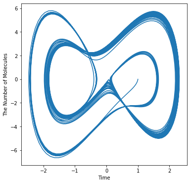
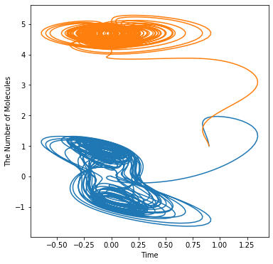
Modified Chua chaotic attractor
[4]:
alpha, beta = 10.82, 14.286
a, b, d = 1.3, 0.1, 0.2

with reaction_rules():
    h = -b * sin(pi * x / (2 * a) + d)
    ~x > x | (alpha * (y - h))
    ~y > y | (x - y + z)
    ~z > z | (-beta * y)

run_simulation(250, ndiv=5000, y0={'x': 0, 'y': 0.49899, 'z': 0.2}).plot(x='x', y='y')
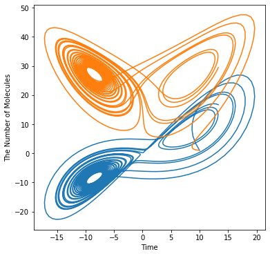
Lorenz system
[5]:
p, r, b = 10, 28, 8.0 / 3

with reaction_rules():
    ~x > x | (-p * x + p * y)
    ~y > y | (-x * z + r * x - y)
    ~z > z | (x * y - b * z)

run_simulation(25, ndiv=2500, y0={'x': 10, 'y': 1, 'z': 1}).plot(x='x', y=['y', 'z'])
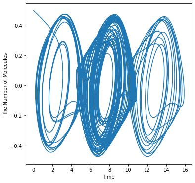
Tamari attractor
[6]:
a = 1.013
b = -0.021
c = 0.019
d = 0.96
e = 0
f = 0.01
g = 1
u = 0.05
i = 0.05

with reaction_rules():
    ~x > x | ((x - a * y) * cos(z) - b * y * sin(z))
    ~y > y | ((x + c * y) * sin(z) + d * y * cos(z))
    ~z > z | (e + f * z + g * a * atan((1 - u) / (1 - i) * x * y))

run_simulation(800, ndiv=8000, y0={'x': 0.9, 'y': 1, 'z': 1}).plot(x='x', y=['y', 'z'])
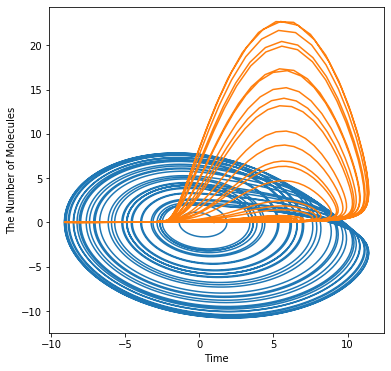
Moore-Spiegel attractor
[7]:
T, R = 6, 20
with reaction_rules():
    ~x > x | y
    ~y > y | z
    ~z > z | (-z - (T - R + R * x * x) * y - T * x)

run_simulation(100, ndiv=5001, y0={'x': 1, 'y': 0, 'z': 0}).plot(x='x', y='y')