Welcome to E-Cell4 in Jupyter Notebook!¶

Quick Start¶

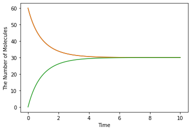
Binding and unbinding reactions¶

Here is an extremely simple example with a reversible binding reaction:

[1]:

%matplotlib inline
from ecell4.prelude import *

with reaction_rules():
    A + B == C | (0.01, 0.3)

run_simulation(10, {'A': 60, 'B': 60})

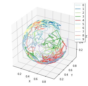
Diffusion on a spherical surface¶

[2]:

%matplotlib inline
from ecell4.prelude import *

with species_attributes():
    M | {'dimension': 2}
    A | {'D': 1.0, 'location': 'M'}

surface = Sphere(ones() * 0.5, 0.49).surface()
obs = FixedIntervalTrajectoryObserver(4e-3)
run_simulation(
    0.4, y0={'A': 10}, structures={'M': surface},
    solver='spatiocyte', observers=obs)

show(obs)

Plotly¶

Interactive visualizations by Plotly are also available. This part might not works on Google Colab.

[3]:

%matplotlib inline
from ecell4.prelude import *

[4]:

with reaction_rules():
    A + B == C | (0.01, 0.3)

ret = run_simulation(10, {'A': 60, 'B': 60})

[5]:

ret.plot(backend='plotly')

[6]:

with species_attributes():
    M | {'dimension': 2}
    A | {'D': 1.0, 'location': 'M'}

ret = run_simulation(
    0.4,
    y0={'A': 10},
    structures={'M': Sphere(ones() * 0.5, 0.49).surface()},
    solver='spatiocyte',
    observers=FixedIntervalTrajectoryObserver(1e-3))

[7]:

plotting.plot_world(ret.world, species_list=['M', 'A'], backend='plotly')

[8]:

plotting.plot_trajectory(ret.observers[1], backend='plotly')

← Installation of the E-Cell... <no title> →