See also
This page was generated from examples/example05.ipynb.
Download the Jupyter Notebook for this section: example05.ipynb. View in nbviewer.
Glycolysis Model and Metabolic Control Analysis
[1]:
%matplotlib inline
from ecell4.prelude import *
A Simple Model of the Glycolysis of Human Erythrocytes
This is a model for the glycolysis of human erythrocytes which takes into account ATP-synthesis and -consumption. This model is based on the model introduced in the following publications:
[2]:
citation(125616)
Heinrich R, Rapoport TA, Mathematical analysis of multienzyme systems. II. Steady state and transient control. Bio Systems, 1(7), 130-6, 1975. 10.1016/0303-2647(75)90050-7. PubMed PMID: 125616.
[3]:
citation(168932)
Rapoport TA, Heinrich R, Mathematical analysis of multienzyme systems. I. Modelling of the glycolysis of human erythrocytes. Bio Systems, 1(7), 120-9, 1975. 10.1016/0303-2647(75)90049-0. PubMed PMID: 168932.
The model consists of seven reactions and is at the steady state.
[4]:
with reaction_rules():
    2 * ATP > 2 * A13P2G + 2 * ADP | (3.2 * ATP / (1.0 + (ATP / 1.0) ** 4.0))
    A13P2G > A23P2G | 1500
    A23P2G > PEP | 0.15
    A13P2G + ADP > PEP + ATP | 1.57e+4
    PEP + ADP > ATP | 559
    # AMP + ATP > 2 * ADP | (1.0 * (AMP * ATP - 2.0 * ADP * ADP))
    AMP + ATP > 2 * ADP | 1.0 * AMP * ATP
    2 * ADP > AMP + ATP | 2.0 * ADP * ADP
    ATP > ADP | 1.46

m = get_model()
[5]:
show(m)
2 * ATP > 2 * A13P2G + 2 * ADP | ((3.2 * ATP) / (1.0 + pow((ATP / 1.0), 4.0)))
A13P2G > A23P2G | 1500.0
A23P2G > PEP | 0.15
A13P2G + ADP > PEP + ATP | 15700.0
PEP + ADP > ATP | 559.0
AMP + ATP > 2 * ADP | (1.0 * AMP * ATP)
2 * ADP > AMP + ATP | (2.0 * ADP * ADP)
ATP > ADP | 1.46
[6]:
y0 = {"A13P2G": 0.0005082, "A23P2G": 5.0834, "PEP": 0.020502,
      "AMP": 0.080139, "ADP": 0.2190, "ATP": 1.196867}
[7]:
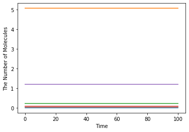
ret = run_simulation(100, model=m, y0=y0)
[8]:
ret
Metabolic Control Analysis
[9]:
import numpy
[10]:
w = ret.world
sim = ode.Simulator(w, m)
First of all, get_stoichiometry gives a stoichiometry matrix from the given species and reactions as follows:
[11]:
numpy.array(get_stoichiometry(m.list_species(), m.reaction_rules()))
[11]:
array([[ 2., -1.,  0., -1.,  0.,  0.,  0.,  0.],
       [ 0.,  1., -1.,  0.,  0.,  0.,  0.,  0.],
       [ 2.,  0.,  0., -1., -1.,  2., -2.,  1.],
       [ 0.,  0.,  0.,  0.,  0., -1.,  1.,  0.],
       [-2.,  0.,  0.,  1.,  1., -1.,  1., -1.],
       [ 0.,  0.,  1.,  1., -1.,  0.,  0.,  0.]])
The evaluate method of ode.ODEWorld returns current fluxes of the given reactions.
[12]:
numpy.array(w.evaluate(m.reaction_rules()))
[12]:
array([1.25489042, 0.76235178, 0.76235178, 1.74742906, 2.50978084,
       0.0959183 , 0.0959183 , 1.74742906])
ode.ODESimulator has methods for the fundamental properties related to metabolic control analysis.
[13]:
x = numpy.array(sim.values())
x
[13]:
array([5.08234520e-04, 5.08234520e+00, 2.05016233e-02, 8.01410043e-02,
       2.18995778e-01, 1.19686922e+00])
[14]:
dxdt = numpy.array(sim.derivatives())
dxdt
[14]:
array([ 0.00000000e+00, -7.32716110e-11, -1.27009514e-13,  1.07631959e-12,
        1.09356968e-12, -2.16981988e-12])
[15]:
J = numpy.array(sim.jacobian())
J
[15]:
array([[-4.93823371e+03,  0.00000000e+00,  0.00000000e+00,
         0.00000000e+00, -7.97928197e+00, -3.54260035e+00],
       [ 1.50000000e+03, -1.50000000e-01,  0.00000000e+00,
         0.00000000e+00,  0.00000000e+00,  0.00000000e+00],
       [ 3.43823371e+03,  1.50000000e-01, -1.22418640e+02,
         0.00000000e+00, -3.48112548e+00,  0.00000000e+00],
       [ 0.00000000e+00,  0.00000000e+00,  0.00000000e+00,
        -1.19686922e+00,  8.75985548e-01, -8.01410043e-02],
       [-3.43823371e+03,  0.00000000e+00, -1.22418640e+02,
         2.39373844e+00, -2.11916605e+01, -1.92231834e+00],
       [ 3.43823371e+03,  0.00000000e+00,  1.22418640e+02,
        -1.19686922e+00,  2.03156750e+01,  2.00245935e+00]])
[16]:
E = numpy.array(sim.elasticity())
E
[16]:
array([[ 0.00000000e+00,  0.00000000e+00,  0.00000000e+00,
         0.00000000e+00,  0.00000000e+00, -1.77130018e+00],
       [ 1.50000000e+03,  0.00000000e+00,  0.00000000e+00,
         0.00000000e+00,  0.00000000e+00,  0.00000000e+00],
       [ 0.00000000e+00,  1.50000000e-01,  0.00000000e+00,
         0.00000000e+00,  0.00000000e+00,  0.00000000e+00],
       [ 3.43823371e+03,  0.00000000e+00,  0.00000000e+00,
         0.00000000e+00,  7.97928197e+00,  0.00000000e+00],
       [ 0.00000000e+00,  0.00000000e+00,  1.22418640e+02,
         0.00000000e+00,  1.14604074e+01,  0.00000000e+00],
       [ 0.00000000e+00,  0.00000000e+00,  0.00000000e+00,
         1.19686922e+00,  0.00000000e+00,  8.01410043e-02],
       [ 0.00000000e+00,  0.00000000e+00,  0.00000000e+00,
         0.00000000e+00,  8.75985548e-01,  0.00000000e+00],
       [ 0.00000000e+00,  0.00000000e+00,  0.00000000e+00,
         0.00000000e+00,  0.00000000e+00,  1.46000000e+00]])
ode.ODESimulator also provides a stoichiometry matrix and fluxes.
[17]:
S = numpy.array(sim.stoichiometry())
S
[17]:
array([[ 2., -1.,  0., -1.,  0.,  0.,  0.,  0.],
       [ 0.,  1., -1.,  0.,  0.,  0.,  0.,  0.],
       [ 0.,  0.,  1.,  1., -1.,  0.,  0.,  0.],
       [ 0.,  0.,  0.,  0.,  0., -1.,  1.,  0.],
       [ 2.,  0.,  0., -1., -1.,  2., -2.,  1.],
       [-2.,  0.,  0.,  1.,  1., -1.,  1., -1.]])
[18]:
v = numpy.array(sim.fluxes())
v
[18]:
array([1.25489042, 0.76235178, 0.76235178, 1.74742906, 2.50978084,
       0.0959183 , 0.0959183 , 1.74742906])
These properties satisfy some relations at the steady state.
\(\frac{\mathrm{d}}{\mathrm{d}t}\mathbf{x} = \mathbf{S} \mathbf{v}\)
[19]:
numpy.isclose(dxdt, S @ v)
[19]:
array([ True, True, True, True, True, True])
\(\mathbf{J} = \frac{\mathrm{d}^2}{\mathrm{d}t^2}\mathbf{x} = \mathbf{S}\left(\frac{\mathrm{d}}{\mathrm{d}t}\mathbf{v}\right) = \mathbf{S} \mathbf{E}\)
[20]:
numpy.isclose(J, S @ E)
[20]:
array([[ True,  True,  True,  True,  True,  True],
       [ True,  True,  True,  True,  True,  True],
       [ True,  True,  True,  True,  True,  True],
       [ True,  True,  True,  True,  True,  True],
       [ True,  True,  True,  True,  True,  True],
       [ True,  True,  True,  True,  True,  True]])
Next, the ecell4.mca submodule provides useful functions for metabolic network and control analyses.
[21]:
from ecell4.mca import *
generate_full_rank_matrix gives square matrix to be full rank. In this model, 5 out of 8 reactions are independent.
[22]:
(link_matrix, kernel_matrix, independent_list) = generate_full_rank_matrix(S)
print(link_matrix)
print(kernel_matrix)
print(independent_list)
[[ 1.  0.  0.  0.  0.]
 [ 0.  1.  0.  0.  0.]
 [ 0.  0.  1.  0.  0.]
 [ 0.  0.  0.  1.  0.]
 [ 0.  0.  0.  0.  1.]
 [ 0.  0.  0. -1. -1.]]
[[-0.  -0.   0.5]
 [-0.  -1.   1. ]
 [-0.  -1.   1. ]
 [-0.   1.   0. ]
 [ 0.   0.   1. ]
 [ 1.   0.   0. ]
 [ 1.   0.   0. ]
 [ 0.   1.   0. ]]
[0 1 2 3 4]
[23]:
reduced_matrix = numpy.take(S, independent_list, 0)
reduced_matrix
[23]:
array([[ 2., -1.,  0., -1.,  0.,  0.,  0.,  0.],
       [ 0.,  1., -1.,  0.,  0.,  0.,  0.,  0.],
       [ 0.,  0.,  1.,  1., -1.,  0.,  0.,  0.],
       [ 0.,  0.,  0.,  0.,  0., -1.,  1.,  0.],
       [ 2.,  0.,  0., -1., -1.,  2., -2.,  1.]])
The original stoichiometry matrix can be reproduced from these reduced matrices:
[24]:
S == link_matrix @ reduced_matrix
[24]:
array([[ True,  True,  True,  True,  True,  True,  True,  True],
       [ True,  True,  True,  True,  True,  True,  True,  True],
       [ True,  True,  True,  True,  True,  True,  True,  True],
       [ True,  True,  True,  True,  True,  True,  True,  True],
       [ True,  True,  True,  True,  True,  True,  True,  True],
       [ True,  True,  True,  True,  True,  True,  True,  True]])
[25]:
0 == S @ kernel_matrix
[25]:
array([[ True,  True,  True],
       [ True,  True,  True],
       [ True,  True,  True],
       [ True,  True,  True],
       [ True,  True,  True],
       [ True,  True,  True]])
Finally, ecell4.mca provides two functions, unscaled_control_coefficients and scaled_control_coefficients, which calculate concentration and flux control coefficients from stoichiometry and elasticity matrices.
[26]:
ccc, fcc = unscaled_control_coefficients(S, E)
print(ccc)
print(fcc)
[[ 4.45754267e-04 -2.22877134e-04  0.00000000e+00 -1.93612289e-04
   0.00000000e+00 -7.45294400e-04  7.45294400e-04 -2.92648441e-05]
 [ 4.45754267e+00  4.43789533e+00 -6.66666667e+00 -1.93612289e+00
   0.00000000e+00 -7.45294400e+00  7.45294400e+00 -2.92648441e-01]
 [ 2.20583561e-02 -2.86048736e-03  0.00000000e+00  1.24794630e-03
  -8.16869067e-03 -4.03592231e-02  4.03592231e-02 -4.10843366e-03]
 [-1.22757774e-01  6.13788871e-02  0.00000000e+00 -2.67777988e-02
   0.00000000e+00 -5.85505375e-01  5.85505375e-01  8.81566859e-02]
 [-1.43377537e-01  7.16887683e-02  0.00000000e+00 -3.12756961e-02
   0.00000000e+00  3.62033276e-01 -3.62033276e-01  1.02964464e-01]
 [ 2.66135311e-01 -1.33067655e-01  0.00000000e+00  5.80534949e-02
   0.00000000e+00  2.23472099e-01 -2.23472099e-01 -1.91121150e-01]]
[[ 5.28594477e-01  2.35702761e-01  0.00000000e+00 -1.02830166e-01
   0.00000000e+00 -3.95836168e-01  3.95836168e-01  3.38532927e-01]
 [ 6.68631401e-01  6.65684300e-01  0.00000000e+00 -2.90418434e-01
   0.00000000e+00 -1.11794160e+00  1.11794160e+00 -4.38972662e-02]
 [ 6.68631401e-01  6.65684300e-01  1.11022302e-16 -2.90418434e-01
   0.00000000e+00 -1.11794160e+00  1.11794160e+00 -4.38972662e-02]
 [ 3.88557554e-01 -1.94278777e-01  0.00000000e+00  8.47581026e-02
   0.00000000e+00  3.26269264e-01 -3.26269264e-01  7.20963121e-01]
 [ 1.05718895e+00  4.71405523e-01  0.00000000e+00 -2.05660332e-01
   0.00000000e+00 -7.91672336e-01  7.91672336e-01  6.77065854e-01]
 [-1.25596650e-01  6.27983250e-02  0.00000000e+00 -2.73970578e-02
   0.00000000e+00  3.17135918e-01  6.82864082e-01  9.01953828e-02]
 [-1.25596650e-01  6.27983250e-02  0.00000000e+00 -2.73970578e-02
   0.00000000e+00  3.17135918e-01  6.82864082e-01  9.01953828e-02]
 [ 3.88557554e-01 -1.94278777e-01  0.00000000e+00  8.47581026e-02
   0.00000000e+00  3.26269264e-01 -3.26269264e-01  7.20963121e-01]]
Unscaled control coefficients satisfies connectivity theorem:
[27]:
numpy.isclose(fcc @ (E @ link_matrix), 0)
[27]:
array([[ True,  True,  True,  True,  True],
       [ True,  True,  True,  True,  True],
       [ True,  True,  True,  True,  True],
       [ True,  True,  True,  True,  True],
       [ True,  True,  True,  True,  True],
       [ True,  True,  True,  True,  True],
       [ True,  True,  True,  True,  True],
       [ True,  True,  True,  True,  True]])
and
[28]:
numpy.isclose(numpy.take(ccc, independent_list, 0) @ (E @ link_matrix), -numpy.identity(link_matrix.shape[1]))
[28]:
array([[ True,  True,  True,  True,  True],
       [ True,  True,  True,  True,  True],
       [ True,  True,  True,  True,  True],
       [ True,  True,  True,  True,  True],
       [ True,  True,  True,  True,  True]])
On the other hand, scaled control coefficients
[29]:
ccc, fcc = scaled_control_coefficients(S, E, v, x)
print(ccc)
print(fcc)
[[ 1.10061937 -0.3343157   0.         -0.6656843   0.         -0.14065824
   0.14065824 -0.10061937]
 [ 1.10061937  0.6656843  -1.         -0.6656843   0.         -0.14065824
   0.14065824 -0.10061937]
 [ 1.35017697 -0.10636707  0.          0.10636707 -1.         -0.18882349
   0.18882349 -0.35017697]
 [-1.92220644  0.58387469  0.         -0.58387469  0.         -0.70077336
   0.70077336  1.92220644]
 [-0.82158249  0.2495576   0.         -0.2495576   0.          0.15856752
  -0.15856752  0.82158249]
 [ 0.27903688 -0.0847581   0.          0.0847581   0.          0.01790928
  -0.01790928 -0.27903688]]
[[ 5.28594477e-01  1.43190526e-01  0.00000000e+00 -1.43190526e-01
   0.00000000e+00 -3.02559747e-02  3.02559747e-02  4.71405523e-01]
 [ 1.10061937e+00  6.65684300e-01  0.00000000e+00 -6.65684300e-01
   0.00000000e+00 -1.40658239e-01  1.40658239e-01 -1.00619373e-01]
 [ 1.10061937e+00  6.65684300e-01  1.11022302e-16 -6.65684300e-01
   0.00000000e+00 -1.40658239e-01  1.40658239e-01 -1.00619373e-01]
 [ 2.79036879e-01 -8.47581026e-02  0.00000000e+00  8.47581026e-02
   0.00000000e+00  1.79092784e-02 -1.79092784e-02  7.20963121e-01]
 [ 5.28594477e-01  1.43190526e-01  0.00000000e+00 -1.43190526e-01
   0.00000000e+00 -3.02559747e-02  3.02559747e-02  4.71405523e-01]
 [-1.64316956e+00  4.99116585e-01  0.00000000e+00 -4.99116585e-01
   0.00000000e+00  3.17135918e-01  6.82864082e-01  1.64316956e+00]
 [-1.64316956e+00  4.99116585e-01  0.00000000e+00 -4.99116585e-01
   0.00000000e+00  3.17135918e-01  6.82864082e-01  1.64316956e+00]
 [ 2.79036879e-01 -8.47581026e-02  0.00000000e+00  8.47581026e-02
   0.00000000e+00  1.79092784e-02 -1.79092784e-02  7.20963121e-01]]
satisfies summation theorem:
[30]:
numpy.isclose(ccc.sum(axis=1), 0)
[30]:
array([ True, True, True, True, True, True])
and
[31]:
numpy.isclose(fcc.sum(axis=1), 1)
[31]:
array([ True, True, True, True, True, True, True, True])